CS 486

Professor Alice Gao, Spring 2019

Lecture 1

Applications of AI:

checkers
chess
go
Jeopardy

Topics in this course:

Search: Heuristic
Supervised Learning
Reasoning under uncertainty
Learning under uncertainty
Decision making under uncertainty

Describe the four definitions of AI. Explain why we will pursue one over the other three.

Cognitive Modeling Approach
- Model human thoughts through brain imaging, cognitive science, etc.
- Systems that think like humans
Turing Test Approach
- See if a human judge can distinguish a robot from a computer
- Systems that act like humans
Laws of Thought Approach
- Laws of logic
- Systems that think rationally
Rational Agent Approach
- Rational agent has rational behavior e.g. learning, having goals
- Rational behavior means to take an action that maximizes the best outcome
- Systems that act rationally

A system is intelligent if it acts rationally.

We pursue the rational agent approach because humans are not necessarily rational (excludes 1 and 2) and laws of logic are hard to translate/apply (excludes 3).

Rationality is mathematically well-defined and completely general.

Lecture 2

sensor ⇒ perceives the environment e.g. mouse, eyes

act ⇒ acts on the environment e.g. monitor, hands, feet

rational agent: selects an action that maximizes its performance measure given a percept sequence and prior knowledge (e.g. rules)

properties of a task environment:

fully observable vs. partially observable (uncertainty) e.g. chess vs. poker (hands of other players are not observed)
deterministic vs. stochastic (uncertain dynamics) e.g. chess (if we know what move the opponent is going to make e.g. opponent is a computer) vs. poker (next card flipped is random)
static vs. dynamic (changing environment) e.g. chess vs. medical diagnostic
episodic vs. sequential (long term consequences of actions) e.g. imagic classification vs. crossword
known vs. unknown (agent knows the rules of the environments) e.g. chess vs. playing chess for the first time
single agent vs. multi-agent e.g. crossword vs. autonomous cars (when you model other cars)

We can formulate real world problems as search problems.

N Queens

states: 16C8 positions for the queens
start state: any of those states
goal test: are the queens attacking each other?
action: move 1 queen away (in any valid direction) from attacking queen, cost of movement is 0
successor function: valid actions

River Crossing

states: who is on either side of the river
start state: parent and children are on left side of the river
goal state: parent and children are on the right side of the river
successor function: move up to 100kg of weight across the river

Propositional satisfiability

states: truth values of each boolean variable used in the expression
start state: all false
goal state: expression is true
successor function: try to flip a boolean variable, from right to left

Traveling salesman problem

states: path of salesman
start state: salesman at start city
goal state: salesman goes to every city
successor function: cool

Lecture 3

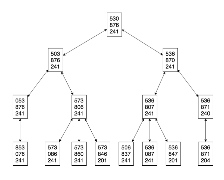
8 Puzzle Problem

state: Each state is given by $x_{00},x_{01},x_{02}, \\ x_{10},x_{11},x_{12}, \\ x_{20},x_{21},x_{22}$ where $x_{ij}$ is the value in the space at column i and row j. If the space is blank, the value is 0. $i, j \in {0, 1, 2}$, $x_{ij} \in {0, \dots, 8}$.

initial state: 530, 876, 241

goal state: 123, 456, 780

action: Move the blank space up, down, left, or right, wherever possible.

successor function: The resulting state after 1 action

cost function: Each move has a cost of 1.

For the 8 puzzle problem, here are the first 4 layers of the search graph:

frontier = []
frontier.append(initial_state)

while frontier:
	# DFS: Expand most recent
	curr_state = frontier.pop()
	# BFS: Expand oldest
	curr_state = frontier.pop(0)
	if curr_state == GOAL_STATE:
		return curr_state
	successors = get_successors(curr_state)
	# Implementation assumes no duplicates
	# If duplicates, remember search tree as hashmap
	frontier += successors

raise Exception("No solution")

Whether we should use BFS or DFS depends on the scenario:

Memory is limited ⇒ DFS
All solutions are deep in the tree ⇒ DFS
The search graph contains cycles ⇒ BFS

If we don’t remember the search tree, DFS gets cycles. BFS also gets stuck in cycles, but it will add its cycle to a queue.
The branching factor is large ⇒ DFS

Assume m is the number of levels, b is the branching factor. Then DFS is O(bm) while BFS is O(b^m).
We must find the shallowest goal node ⇒ BFS
Some solutions are very shallow ⇒ BFS

search graph: contains all states and edges for the successor function

search tree: constructed as we execute the algorithm (tree nodes are 1 directional)

frontier: all leaf nodes available for expansion

expanding a node removes it from the frontier
generating a node adds it to the frontier

Lecture 4

BFS and DFS are uninformed search algorithms. When we can, we should used informed search algorithms like A* search to find the target solution faster.

A* search algorithm

g(n): cost of the path from initial state to current state n, known

search heuristic h(n): estimate of the cost of the cheapest path from node n to a goal node

h(n) ≥ 0. If n is a goal node, h(n) = 0
h(n) must be easy to compute (without search)

informed search algorithm: Same as DFS/BFS, except you treat the frontier as a priority queue ordered by f(n)

Djikstra’s: f(n) = g(n)
Greedy: f(n) = h(n)
A*: f(n) = g(n) + h(n)

A* is optimally efficient because among all optimal algorithms that start from the same start node and use the same heuristic, A* expands the fewest nodes.

admissible heuristic: lower bound optimistic estimate of the cost of getting from node n to the nearest goal node

We verify that a heuristic is admissible by showing that it is an optimal solution to a relaxed version of the problem.

For the 8 puzzle problem, relaxed problems are:

A tile can move from A to B if A and B are adjacent
- Optimal solution is Manhattan distance for each tile
A tile can move from A to B if B is blank
A tile can move from A to B
- Optimal solution is the number of misplaced tiles

To construct an admissible heuristic, relax a search problem and find the optimal solution in the relaxed case.

A heuristic $h_1(n)$ dominates another heuristic $h_2(n)$ if for all states $h_1$ ≥ $h_2$ and for at least 1 state, $h_1$ > $h_2$.

If $h_1$ dominates $h_2$, A* using $h_1$ will never expand more states using $h_1$ than $h_2$. So, we should always choose dominating heuristics.

Other desirable properties:

heuristic admissible, but with high values (close to true h)
not a constant function

Lecture 5

Components of a constraint satisfaction problem (CSP):

A set X of variables
A set D of domains
A set C of constraints specifying allowable combinations of values

A solution to a CSP is a set of assignments to X that satisfy all C.

For the 4 Queens problem:

X = ${x_0, x_1, x_2, x_3}$, where $x_i$ is the row of the the Queen in column i
Domain of $x_i$ is ${0, 1, 2, 3}$
C:
- No 2 queens can be in the same row ⇒ For all i, j where i ≠ j, $x_i$ ≠ $x_j$
- No 2 queens can be in the same diagonal ⇒ For all i, j where i ≠ j, $\vert x_i - x_j \vert ≠ 2$
- No 2 queens can be in the same column ⇒ Not necessary since this is impossible by the formulation of X

For the 4 queens problem, we have the constraint: The queens in columns 0 and 2 are not in the same row or diagonal.

In table format:

$x_0$	$x_1$
0	1
0	3
1	0
1	2

In formula format:

\[(x_0 \ne x_2) \land (|x_0 - x_2| \ne 2)\]

arc-consistency: $X_i$ is arc-consistent with respect to another variable $X_j$ if and only if for every value $c_i$ in $D_i$, there is a value $v_j$ in $D_j$ such that $(v_i, v_j)$ satisfies the constraint $(X_i, X_j)$.

Arc consistency algorithm

def revise(X_i, C):
	revised = False
	for x in dom(X_i):
		if not exists y in dom(X_i s.t. (x, y) satisfies C:
			remove x from dom(X_i)
			revised = True
	return revised

def ac3(X, D, C):
	Put (v, C) in the set S for every variable v and every constraint involving v
	while S:
		X_i, C_ij = S.pop()
		if revise(X_i, Cij):
			if not dom(X_i): 
				return False
			# For all constraints where X_i is the other variable
			for X_k where C_ki is a constraint between X_k and X_i:
				# Adds if X_k, C_ki is not already in S
				S.add((X_k, C_ki))

3 possible outcomes to the arc-consistency algorithm:

no solution
1 unique solution
multiple solutions

Complexity of the arc consistency algorithm

Assume $n$ variables, $c$ binary constraints, and the size of the domain at each step is at most $d$. Then the complexity is $O(ncd)$.

The algorithm always terminate because we shrink the domain at each step.

arity: the number of variables involved in a constraint

Lecture 6, 7

local search: keep track of a single node, move to a neighbor of the node based on how good the neighbor is

Advantages over other search algorithms:

Can be used when state space is large or infinite
Doesn’t use a lot of memory (only stores 1 state)
Can solve pure optimization problems where there is no goal state to test against
Good for solving CSPs, since path to goal state in CSP is irrelevant.

Components of a local search problem:

A set of variables
Domains for variables
Constraints on the joint values of variables
Node: a complete assignment to all of the variables
Neighbor relation for each node
- If the neighborhood at each step
  - large, we get large improvements at each step, less likely to get stuck
  - small, we get small improvement at each step, faster
Cost function for each node

For the 4 queens problem:

state: 4 queens on the board
- Variables: $x_0, x_1, x_2, x_3$
- Domain for each variable: $x_i \in {0, 1, 2, 3}$
initial state: Any random state
goal state: No pair of queens attacking each other
neighbor relation:
- Version A: Move a single queen to another square in the same column
- Version B: Swap the row positions of two queens
cost function: The number of pairs of queens attacking each other directly or indirectly

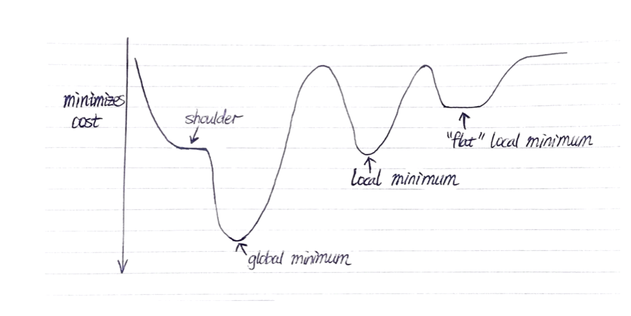
local optima: a state s* is locally optimal if c(s) ≤ c(s) for every state s in the neighborhood of s

global optima: a state s* is globally optimal if c(*) ≤ c(s) for every state s

plateau: flat area in the state space

shoulder: possible to improve when we escape
flat local optimum: cannot improve even if we escape

Strategies for escaping local optima

sideway moves ⇒ allow max number of moves to neighbors with the same cost
taboo list ⇒ keep a small list of recently visited states and forbid the algorithm to return to those states
hill climbing with random restarts ⇒ restart search in different part of the state space
- finds optimal solution given enough restarts
hill climbing with simulated annealing ⇒ move to a state with high cost occasionally
1. Start with a random solution and a large T.
2. Choose a random neighbor. If the neighbor is better than current move to the neighbor. If the neighbor is not better than the current state, move to the neighbor with probability $p = e^{\frac{\Delta E}{T}}$ where $E = \text{cost}(current) - \text{cost}(next)$. Define lower $\text{cost(x)}$ to be better.
3. Stop when T = 0. If T decreases slowly enough, simulated annealing is guaranteed to fin the global optimum.

Comparing hill climbing with genetic algorithms:

Exploring state space
- Hill climbing explores neighbors of the state based on neighbor relation
- Genetic algorithm uses mutation/reproduction to explore
Optimizing quality of state/population
- Hill climbing chooses the best neighbor
- Genetic algorithm chooses best parents

Parallel search

Maintain k nodes, update each one independently
Equivalent to doing k random restarts in parallel

Beam search

Maintain k nodes, choose k best nodes out of all the neighbors
When k = 1, hill climbing
Loses diversity very fast if all k neighbors in the same area

Stochastic beam search

Beam search, but k best nodes are chosen with a probability proportional to fitness of the node
Maintains diversity

Genetic algorithm

Keep track of a set of states. Each state has a fitness.
Randomly two states to reproduce. The fitter a state, the more likely it’s chosen to reproduce
Two parent states cross over to produce a child state
The child state mutates with a small independent probability
Add the child state to the new population
Repeat reproduction until we produce a new population. Replace the old population with the new one
Repeat until one state in the population has high enough fitness.

Lecture 8, 9

Reasons for building an agent that can learn

Don’t know the solution ourselves
World evolves, cannot anticipate all changes over time
Cannot anticipate all possible situations

Different types of learning

unsupervised learning: learn patterns in the examples, no labels available
semi-supervised learning: learn from a few labeled examples and a large number of unlabelled examples
supervised learning: learn a function that maps from examples to labels

supervised learning:

training set of (x, y) pairs generated by some unknown function f(x) = y
find a function h in hypothesis space H that approximates f
- Choose h that is most accurate on the test set of examples ⇒ h that generalizes best
- We want the simplest consistent hypothesis

classification: label is a discrete value

regression: label has continuous values

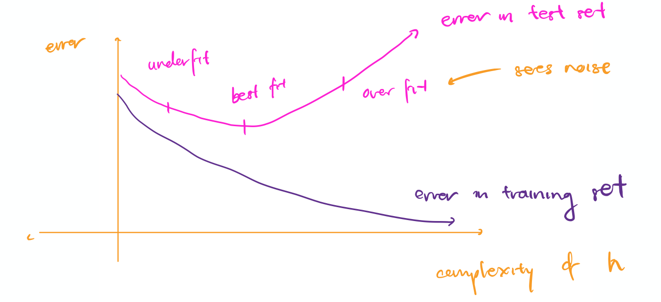
overfitting: h that fits training data too well and does not generalize to test set

decision tree: graph of nodes, at each node divide up examples based on the value for a chosen feature

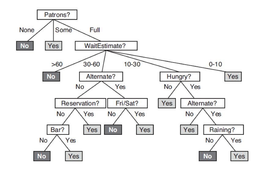
We construct a decision tree by testing features in order until each leaf contains training examples with the same label. The resulting tree will fit the training set perfectly.

We want an order of testing features that gives a tree that is as shallow (simple) as possible.

def ID3(features, examples):
	If all examples are positive, return a leaf node with decision yes
	If all examples are negative, return a leaf node with decision no
	# If there are hidden features or data is noisy
	If no features left, return a leaf node with the majory decision of the examples
	# If training data doesn't contain this combination of values
	If no examples left, return a leaf node with the majority decision of the examples in the parent
	
	# Choose the feature with greatest information gain
	Choose the most important feature f
	for each value v of feature f:
		add arc with label v
		add subtree ID3(F - f, s in S | f(s) = v)

entropy of distribution with k outcomes: $I(P(c_1) \dots P(c_k) = -\sum^{k}_{i = 1} P(c_i)\log_2 P(c_i)$

maximum entropy = 1 when distribution is even between classes
Define I(1, 0) = 0, I(0, 1) = 0

Expected information gain for selecting a feature

Before testing a feature, suppose there are p positive examples and n negative examples.

Entropy before testing the feature:

$E_0 = I(\frac{p}{p + n}, \frac{n}{p + n})$ Expected entropy after testing the feature:

$E_1 = \sum^k_{i = 1} \frac{p_i + n_i}{p + n} \cdot I(\frac{p_i}{p_i + n_i}, \frac{p_i}{p_i + n_i})$ Expected information gain after testing the feature:

\[G = E_0 - E_1\]

Lecture 10

Decision trees with real-value features

To choose a split point for a real valued feature:

Sort the instances according to the real valued feature
Call every value halfway between two adjacent instance values a possible split point. If there exist at least 1 pair of labels with differing values on either side of the split point, record its expected information gain.
Pick the split point with the maximum information gain.

We can test a real valued features multiple times, but discrete valued features a maximum of once. This makes computing real valued decision trees expensive.

Preventing overfitting in decision trees

To get a smaller tree to prevent overfitting to noisy data:

Grow the tree to a maximum depth
Enforce a minimum number of examples at a leaf node
Post-prune the tree using a validation set

Choose the best maximum depth of decision tree by k-fold cross validation

Use k-fold cross validation to split the dataset into k pairs of training sets and validation sets. Train k trees of a given depth. The accuracy for that depth is the average accuracy between the k trees.
Do k-fold cross validation several times to pick the best maximum depth.

Lecture 11

Causes and resolutions of the two AI winters:

1970s - 1980s
- 1969 → Marvin Minsky proved we need to use multi-layer perceptrons to represent simple non-linear functions such as XOR
- Unclear how to train multi-layer perceptrons
  - 1986 → Rumelhart, Hinton, and Williams use back-propagation to train multi-layer perceptrons
mid 1990s
- Multi-layer neural networks trained with back propagation don’t work well compared to simpler models
- Rise of deep learning
  - 2006 → Hinton, Osindero, and Teh show that back-propagation works if initial weights are chosen in a smart way
  - 2012 → Hinton enters ImageNet competition using deep convolutional neural networks and did far better than the next closest entry

4 lessons learned summarized by Geoff Hinton

Labelled data sets were thousands of times too small
Our computers were millions of times too slow
We initialized the weights in a stupid way
We used the wrong type of non-linearity (relu better than sigmoid).

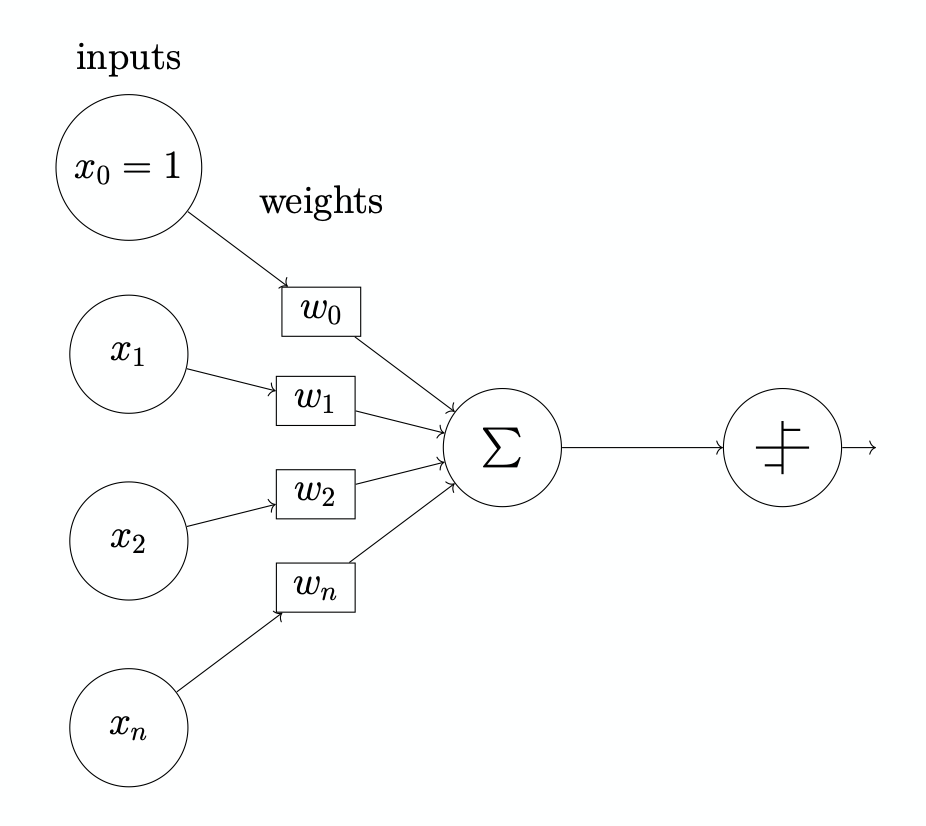
A drawn simple perceptron:

Lecture 12

$P(X)$ ⇒ prior, unconditional, likelihood of X given background information

$P(X \vert Y)$ ⇒ posterior, conditional, likelihood of X given Y

random variable

has a domain of possible values
has an associated probability distribution

probabilistic model: a set of random variables

atomic event: assigns a value to every ranom variable in the model

joint probability distribution: assigns a probability to every atomic event

Sum rule: $P(X = x \land Y = y) = \sum_{z = \{T, F\}} P(X = x \land Y = y \land Z = z)$ Product rule:

$P(X = x \vert Y = y) = \frac{P(X=x \land Y = y}{P(Y = y)}$ Chain Rule:

$P(A, B, C) = P(A \vert B, C) \cdot P(B \vert C) \cdot P(C)$ Bayes Rule:

\[P(X \vert Y) = \frac{P(Y \vert X) \cdot P(X)}{P(Y)}\]

Lecture 13

independence: $X$ is independent of $Y$ if $P(X \vert Y) = P(X)$

conditional independence: $X$ is conditionally independent of $Y$ if $P(X \vert Y, Z) = P(X \vert Z)$

Computing a joint probability given a Bayesian network:

Choose an order of the variables consistent with the partial ordering in the Bayesian Network
Compute the joint probability using the formula $P(X_n, \dots, X_1) = \prod^n_{i = 1} P(X_i \vert Parents(X_i))$

Markov blanket: the node’s parents, children, and other parents of children

In a Bayesian network, a node is conditionally independent of all other nodes given the node’s Markov Blanket.

Lecture 16

Markov model:

Each world contains a series of time slices
Each time slice t contains X, unobservable state variables and E, observable evidence variables
Markov assumption: The current state only depends on a fixed number of previous states
First order Markov process: every variable only depends on previous state

PREVIOUSENGL 108D

NEXTENGL 315