
Markdown transcription of my handwritten CS 370 notes. Spelling and wording are preserved where legible; diagrams are described in brackets, and editorial clarifications are also in brackets.
Floating Point
Normalized form of a real number $F=\lbrace\beta,t,L,U\rbrace$:
\[0.d_1d_2d_3\ldots d_t\times\beta^p\]where $d_i$ are digits in base $\beta$ ($0\leq d_i<\beta$), $d_1\neq0$, and $p$ is an integer where $L\leq p\leq U$.
\[\begin{aligned} \beta&=\text{base}, & L&=\text{lower limit on exponent }p,\\ t&=\text{number of digits}, & U&=\text{upper limit on exponent }p. \end{aligned}\]- IEEE single precision: $\lbrace2,24,-126,127\rbrace$
- IEEE double precision: $\lbrace2,53,-1022,1023\rbrace$
- If $p>U$: overflow.
- If $p<L$: underflow.
Question: For $F=\lbrace2,3,-1,2\rbrace$, list the first six numbers.
Answer:
- $0$
- $0.100_2\times2^{-1}=0.25$
- $0.101_2\times2^{-1}=0.3125$
- $0.110_2\times2^{-1}=0.375$
- $0.111_2\times2^{-1}=0.4375$
- $0.100_2\times2^1=1$
Notice that numbers are not evenly spaced as they would be in fixed-point representation, e.g. $0.001,0.002,0.003$, etc.
Rounding Modes for FP Conversion
Rounding modes for FP conversion:
- Round to nearest number available in $F$ ($0.5$ rounds up).
- Truncation: discard all digits after the $t$th.
Question: Convert:
- $253.9$ to $\lbrace10,6,-5,5\rbrace$
- $8.25$ to $\lbrace2,7,-5,5\rbrace$
- $1030.9671$ to $\lbrace10,6,-5,5\rbrace$
Answer:
\[\begin{aligned} 253.9&=0.2539\times10^3=0.253900\times10^3,\\ 8.25\text{ in base 2}&=1000.01_2=0.1000010_2\times2^4,\\ 1030.9671&=0.10309671\times10^4. \end{aligned}\]For the third number:
- With rounding: $0.103097\times10^4$.
- With truncation: $0.103096\times10^4$.
$x_{\text{exact}}$ means the true solution. $x_{\text{approx}}$ means the approximate, representable solution.
\[E_{\text{abs}}=|x_{\text{exact}}-x_{\text{approx}}|, \qquad E_{\text{rel}}=\frac{|x_{\text{exact}}-x_{\text{approx}}|}{|x_{\text{exact}}|}.\]Question: Compute $E_{\text{abs}}$ and $E_{\text{rel}}$ for $x_{\text{exact}}=220$, $x_{\text{approx}}=198$.
Answer:
\[E_{\text{abs}}=22, \qquad E_{\text{rel}}=\frac{2}{220}=9.\overline{09}\times10^{-3}.\]Relative error is more useful and independent of magnitude.
A result is correct to approximately $s$ digits if
\[0.5\times10^{-s}\leq E_{\text{rel}}<5\times10^{-s},\]or equivalently
\[5\times10^{-(s+1)}\leq E_{\text{rel}}<5\times10^{-s}.\]Therefore,
\[5\times10^{-3}\leq9.\overline{09}\times10^{-3}<5\times10^{-2},\]so about two digits are correct.
Question: Compute the number of digits correct for:
- $E_{\text{rel}}=0.8\times10^{-3}$
- $E_{\text{rel}}=4\times10^2$
Answer:
For (1),
\[5\times10^{-4}\leq0.8\times10^{-3}<5\times10^{-3},\]so three digits are correct.
For (2),
\[5\times10^{-(-2+1)}\leq4\times10^2<5\times10^{-(-2)},\]that is,
\[5\times10^1\leq4\times10^2<5\times10^2,\]so $-2$ digits are correct.
For an FP system $F$, $E_{\text{rel}}$ is bounded such that for any $x\in\mathbb R$ and its FP representation $\operatorname{fl}(x)$,
\[(1-E)|x|\leq|\operatorname{fl}(x)|\leq(1+E)|x|,\]where $E$ is machine epsilon and is defined as the smallest number such that
\[\operatorname{fl}(1+E)>1.\]Therefore,
\[\operatorname{fl}(x)=x(1+\delta)\quad\text{for some }|\delta|\leq E.\]For an FP system $F=\lbrace\beta,t,L,U\rbrace$:
- Under rounding, $E=\frac12\beta^{1-t}$.
- Under truncation, $E=\beta^{1-t}$.
Question: What is $E$ for $F=\lbrace10,3,-5,5\rbrace$?
Answer:
Consider the smallest representable number greater than or equal to $1$ in FP.
\[1=0.100\times10^1.\]The next larger number should be $0.101\times10^1=1.01$, so $E=0.01=1\times10^{-2}$. However, notice under rounding that…
\[1.005\approx1.01,\]so $E=0.005=5\times10^{-3}$ suffices. Thus,
\[E=\frac12(10)^{1-3}=\frac12(10^{-2})=5\times10^{-3}\]is correct for rounding, and
\[E=(10)^{1-3}=10^{-2}=1\times10^{-2}\]is correct for truncation.
IEEE requires that
\[w\oplus z=\operatorname{fl}(w+z)=(w+z)(1+\delta).\]Here $w+z$ is the exact real result represented as FP. But in sequences of operations, error compounds:
\[(a\oplus b)\oplus c\neq a\oplus(b\oplus c)\neq\operatorname{fl}(a+b+c).\]Question: What is the worst relative error for $(a\oplus b)\oplus c$?
Answer:
\[\begin{aligned} E_{\text{rel}} &=\frac{|x_{\text{exact}}-x_{\text{approx}}|}{|x_{\text{exact}}|}\\ &=\frac{|x_{\text{approx}}-x_{\text{exact}}|}{|x_{\text{exact}}|}\\ &=\frac{|(a+b)(1+\delta_1)\oplus c-[a+b+c]|}{|a+b+c|}\\ &=\frac{|[(a+b)(1+\delta_1)+c](1+\delta_2)-a-b-c|}{|a+b+c|}\\ &=\frac{|[a+b+\delta_1(a+b)+c](1+\delta_2)-a-b-c|}{|a+b+c|}\\ &=\frac{|\delta_1(a+b)+\delta_1\delta_2(a+b)+\delta_2(a+b+c)|}{|a+b+c|}. \end{aligned}\]By the triangle inequality, this is less than
\[\frac{|\delta_1(a+b)|}{|a+b+c|} +\frac{|\delta_1\delta_2(a+b)|}{|a+b+c|} +\frac{|\delta_2(a+b+c)|}{|a+b+c|}.\]Since $\lvert\delta_1\rvert\leq E$ and $\lvert\delta_2\rvert\leq E$,
\[E_{\text{rel}} \leq\frac{|a+b|}{|a+b+c|}E +\frac{|a+b|}{|a+b+c|}E^2+E \leq\frac{|a|+|b|}{|a+b+c|}(E^2+E)+E.\]Symmetrically, $E_{\text{rel}}$ for $a\oplus(b\oplus c)$ is
\[E_{\text{rel}} \leq\frac{|b+c|}{|a+b+c|}(E^2+E)+E \leq\frac{|b|+|c|}{|a+b+c|}(E^2+E)+E.\]Therefore, the general bound on $a\oplus b\oplus c$ is
\[\begin{aligned} E_{\text{rel}} &\leq\frac{|a|+|b|+|c|}{|a+b+c|}(E^2+E) +\frac{|a+b+c|}{|a+b+c|}E\\ &\leq\frac{|a|+|b|+|c|}{|a+b+c|}(E^2+E) +\frac{|a|+|b|+|c|}{|a+b+c|}E\\ &\leq\frac{|a|+|b|+|c|}{|a+b+c|}(E^2+2E). \end{aligned}\]$E_{\text{rel}}$ can become very large when
\[|a+b+c|\ll|a|+|b|+|c|.\]This can happen when $a,b,c$ have differing signs, leading to cancellation.
Question: Compute $(a\oplus b)\oplus c$ with $a=2000$, $b=-3.234$, $c=-2000$ for $F=\lbrace10,4,-10,10\rbrace$ with rounding. Find the error bound.
Answer:
\[\begin{aligned} a\oplus b &=2000-3.234=1996.766\\ &=0.1996766\times10^4\\ &\Rightarrow0.1997\times10^4,\\ (a\oplus b)\oplus c&\Rightarrow1997-2000=-3. \end{aligned}\]This is catastrophic cancellation error.
\[(a\oplus b)\oplus c=-0.3000\times10^1, \qquad a+b+c=-0.3234\times10^1.\] \[E_{\text{rel}}=0.072=7.2\times10^{-2},\]so one digit is correct.
From the formula for the error bound of $a\oplus b\oplus c$,
\[E_{\text{rel}} \leq\frac{|a|+|b|+|c|}{|a+b+c|}(2E+E^2) =1.238,\]so the bound guarantees zero digits right, where
\[E=\frac12\beta^{1-t}=\frac12(10)^{1-4}=5\times10^{-4}.\]Question: Compute $(a\oplus c)\oplus b$ for $a=2000$, $b=-3.234$, $c=-2000$, where $F=\lbrace10,4,-10,10\rbrace$. Find the error bound.
Answer:
\[a\oplus c\Rightarrow2000-2000=0.\]This is benign cancellation. Therefore,
\[(a\oplus c)\oplus b\Rightarrow0-3.234=-0.3234\times10^1=a+b+c,\]so $E_{\text{rel}}=0$. The error bound is $1.238$, as before.
Question: Compute $(a\oplus b)\oplus c$ for $a=-2000$, $b=-3.234$, $c=-2000$, where $F=\lbrace10,4,-10,10\rbrace$ with rounding. Find the error bound.
Answer:
\[\begin{aligned} a\oplus b &\Rightarrow-2000-3.234=-2003.234\\ &=-0.2003234\times10^4\\ &\Rightarrow-0.2003\times10^4,\\ (a\oplus b)\oplus c &\Rightarrow-0.2003\times10^4-2000=-4003\\ &=-0.4003\times10^4. \end{aligned}\]Thus $E_{\text{rel}}=5.845\times10^{-5}$, which is a much better error.
\[\text{Error bound} =\frac{|a|+|b|+|c|}{|a+b+c|}(2E+E^2) =10^{-3}.\]The error bound is much better when cancellation is avoided.
Catastrophic cancellation error: subtracting input numbers with error of about the same magnitude.
Benign cancellation: subtracting input numbers with no error of about the same magnitude.
Rules of thumb:
- Sum numbers of the same sign and magnitude.
- If input numbers contain error, reformulate to avoid cancellation.
Consider two formulas for the Taylor series for $e^x$, where $x<0$:
\[\text{i.}\quad e^x\approx1+x+\frac{x^2}{2!}+\frac{x^3}{3!}+\cdots\] \[\text{ii.}\quad e^x\approx\frac1{e^y} =\frac1{1+y+y^2/2!+y^3/3!+\cdots}, \qquad y=|x|.\]The second is much better because it avoids cancellation.
Compare
\[f(x)=\frac{1-\cos^2x}{x^2} \quad\text{and}\quad g(x)=\frac{\sin^2x}{x^2}\]as $x\to0$.
\[\lim_{x\to0}\frac{1-\cos^2x}{x^2} =\lim_{x\to0}\frac{\sin^2x}{x^2}=1,\]but $f(x)$ approximates this much worse because $\cos^2x\approx1$.
Other types of error:
- round-off error (FP representation);
- truncation error (i.e. after $n$ terms of Taylor);
- uncertainty/error in input;
- error/approximation in the model of the situation.
Conditioning and Stability
For a problem $P$ with input $I$ and output $O$, if small $\Delta I$ results in small $\Delta O$, then $P$ is well-conditioned. Otherwise, $P$ is ill-conditioned.
If an algorithm is unstable, any error in the input is magnified.
Conditioning and stability are independent properties.
Question: Analyze the stability of using the recursive algorithm
\[I_0=\log\frac{1+\alpha}{\alpha}, \qquad I_n=\frac1n-\alpha I_{n-1}\quad\text{for }n\geq0\]to approximate
\[I_n=\int_0^1\frac{x^n}{x+\alpha}\,dx.\]Assume some error $E_0$ in $I_0$, i.e.
\[E_0=(I_0)_A-(I_0)_E.\]What is $E_n$ after $n$ steps? Does $E_n$ grow?
Answer:
Both exact and approximate follow the recurrence relation. Therefore,
\[\begin{aligned} E_n &=(I_n)_A-(I_n)_E\\ &=\left[\frac1n-\alpha(I_{n-1})_A\right] -\left[\frac1n-\alpha(I_{n-1})_E\right]\\ &=-\alpha\left[(I_{n-1})_A-(I_{n-1})_E\right]\\ &=(-\alpha)^n\left[(I_0)_A-(I_0)_E\right]\\ &=(-\alpha)^nE_0. \end{aligned}\]Therefore, if $\lvert\alpha\rvert\leq1$, then the algorithm is stable.
Intro to Interpolation
Given a set of data points from an unknown function $y=p(x)$, can we approximate $p$’s value at other points?
Univalence theorem: Given $n$ pairs $(x_i,y_i)$ where $1\leq i\leq n$, there exists a unique polynomial $p(x)$ of degree $\leq n-1$ that interpolates the data.
For $n$ points, find all coefficients $c_i$ of
\[p(x)=c_1+c_2x+c_3x^2+c_4x^3+\cdots+c_nx^{n-1}.\]Plugging in each $(x_i,y_i)$ gives one linear equation:
\[y_i=c_1+c_2x_i+c_3x_i^2+c_4x_i^3+\cdots+c_nx_i^{n-1}.\]This gives an $n\times n$ linear system,
\[\begin{bmatrix} 1&x_1&x_1^2&\cdots&x_1^{n-1}\\ 1&x_2&x_2^2&\cdots&x_2^{n-1}\\ \vdots&\vdots&\vdots&&\vdots\\ 1&x_n&x_n^2&\cdots&x_n^{n-1} \end{bmatrix} \begin{bmatrix}c_1\\c_2\\\vdots\\c_n\end{bmatrix} = \begin{bmatrix}y_1\\y_2\\\vdots\\y_n\end{bmatrix},\]or $V\vec c=\vec y$, where $V$ is the Vandermonde matrix.
\[\det V=\prod_{i<j}(x_i-x_j)\neq0,\]which means there must be a solution. This proves the univalence theorem.
Monomial form:
\[p(x)=c_1+c_2x+c_3x^2+\cdots+c_nx^{n-1} =\sum_{i=1}^nc_ix^{i-1}.\]Monomial basis functions: $1,x,x^2,\ldots$
Lagrange Basis Function
$L_k(x)$:
\[L_k(x)= \frac{(x-x_1)\cdots(x-x_{k-1})(x-x_{k+1})\cdots(x-x_n)} {(x_k-x_1)\cdots(x_k-x_{k-1})(x_k-x_{k+1})\cdots(x_k-x_n)}.\]There is no $x-x_k$ or $x_k-x_k$ entry.
Notice:
\[L_i(x_j)=1\text{ where }i=j\]since numerator/denominator $=1$, and
\[L_i(x_j)=0\text{ where }i\neq j\]since $x_j-x_j$ will occur in the numerator.
Lagrange Form
\[p(x)=y_1L_1(x)+y_2L_2(x)+\cdots+y_nL_n(x) =\sum_{k=1}^ny_kL_k(x).\]$p(x)$ interpolates each $(x_i,y_i)$ by definition. For example,
\[p(x_i)=y_1L_1(x_i)+\cdots+y_iL_i(x_i)+\cdots+y_nL_n(x_i)=y_i.\]Question: Find the Lagrange polynomial $p(x)$ interpolating $(x_1,y_1)=(1,2)$ and $(x_2,y_2)=(-1,4)$.
Answer:
\[L_1(x)=\frac{x-x_2}{x_1-x_2}=\frac{x-(-1)}{1-(-1)}=\frac{x+1}{2},\] \[L_2(x)=\frac{x-x_1}{x_2-x_1}=\frac{x-1}{-1-1}=\frac{x-1}{-2}=\frac{1-x}{2}.\]Therefore,
\[p(x)=2\left(\frac{x+1}{2}\right)+4\left(\frac{1-x}{2}\right) =x+1+2-2x=3-x.\]No need to solve a linear system!
Runge’s Phenomenon
Fitting a high-degree polynomial (many points) often gives excessive oscillation.
We solve this with piecewise functions.
Hermite Interpolation
Fit a cubic to each interval given values and derivatives at each point.
We use the same strategies as in Vandermonde to determine the coefficients of each cubic.
Question: Fit a cubic function $p(x)=a+bx+cx^2+dx^3$ given Hermite data for two points:
\[p(x_1)=y_1,\quad p'(x_1)=s_1, \qquad p(x_2)=y_2,\quad p'(x_2)=s_2.\]Answer:
Plugging into $p(x)$,
\[\begin{aligned} y_1&=a+bx_1+cx_1^2+dx_1^3,\\ y_2&=a+bx_2+cx_2^2+dx_2^3. \end{aligned}\]We know $p’(x)=b+2cx+3dx^2$, so
\[\begin{aligned} s_1&=b+2cx_1+3dx_1^2,\\ s_2&=b+2cx_2+3dx_2^2. \end{aligned}\]Thus,
\[\begin{bmatrix} 1&x_1&x_1^2&x_1^3\\ 1&x_2&x_2^2&x_2^3\\ 0&1&2x_1&3x_1^2\\ 0&1&2x_2&3x_2^2 \end{bmatrix} \begin{bmatrix}a\\b\\c\\d\end{bmatrix} = \begin{bmatrix}y_1\\y_2\\s_1\\s_2\end{bmatrix}.\]If we had $n$ points, we would have to solve $n-1$ of these systems, or $(n-1)(4)=4n-4$ equations. We can skip this work by using the Hermite closed form.
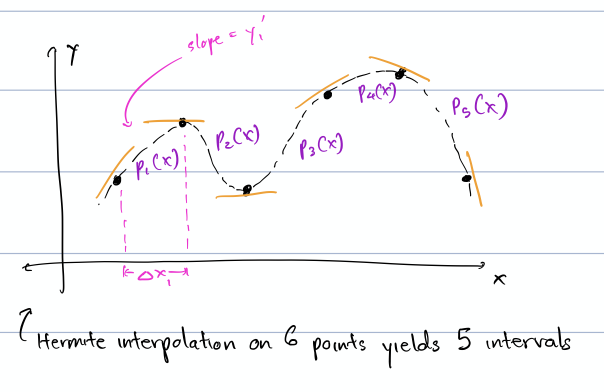
Hermite interpolation on six points yields five intervals. Cubics $p_1(x)$ through $p_5(x)$ join at the data points with prescribed slopes.
Define $p_i(x)$ as the polynomial on the $i$th interval, between points $x_i$ and $x_{i+1}$:
\[p_i(x)=a_i+b_i(x-x_i)+c_i(x-x_i)^2+d_i(x-x_i)^3,\]where
\[\begin{aligned} a_i&=y_i,& \Delta x_i&=x_{i+1}-x_i,\\ b_i&=s_i,& y_i'&=\frac{y_{i+1}-y_i}{\Delta x_i},\\ c_i&=\frac{3y_i'-2s_i-s_{i+1}}{\Delta x_i},&&\\ d_i&=\frac{s_{i+1}+s_i-2y_i'}{(\Delta x_i)^2}.&& \end{aligned}\]$y_i’$ refers to the linear slope, not derivative $s_i$.
Question: Find the Hermite polynomial for $x_1=0$, $y_1=0$, $s_1=1$, $x_2=1$, $y_2=3$, $s_2=0$.
Answer:
\[a_1=y_1=0,\qquad b_1=s_1=1,\] \[\Delta x_1=x_2-x_1=1, \qquad y_1'=\frac{3-0}{1}=3,\] \[c_1=\frac{3(3)-2(1)-0}{1}=7, \qquad d_1=\frac{0+1-2(3)}{1^2}=-5.\]Therefore,
\[p_1(x)=0+1(x-0)+7(x-0)^2-5(x-0)^3=x+7x^2-5x^3.\]Knots: points where the interpolant transfers from $p_i(x)$ to $p_{i+1}(x)$.
Nodes: points where data for the interpolant is specified, i.e. slope.
Hermite interpolation removes discontinuities at each control point by definition, since it creates some polynomial $p_i(x)$ with derivatives $s_i,s_{i+1}$ at each control point. Therefore it creates a smooth curve.
Cubic Splines
Fit a cubic $S_i(x)$ on each interval; require matching first and second derivatives; require only points as input.
For each interval $[x_i,x_{i+1}]$ for $S_i(x)$ and $S_{i+1}(x)$:
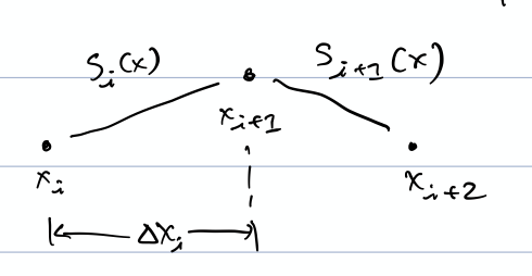
$S_i(x)$ joins $S_{i+1}(x)$ at $x_{i+1}$; the interval from $x_i$ to $x_{i+1}$ is $\Delta x_i$.
Require:
\[\begin{aligned} S_i(x_i)&=y_i, &(1)\\ S_i(x_{i+1})&=y_{i+1}, &(2)\\ S_i'(x_{i+1})&=S_{i+1}'(x_{i+1}), &(3)\\ S_i''(x_{i+1})&=S_{i+1}''(x_{i+1}). &(4) \end{aligned}\]Two equations are needed for boundary conditions $(x_1,x_n)$:
- Clamped: $S’(x_1)=c_1$ and $S’(x_n)=c_2$, where $c_1,c_2$ are given constants.
- Free: $S’‘(x_1)=S’‘(x_n)=0$.
- Periodic: $S_1’(x_1)=S_n’(x_n)$ and $S_1’‘(x_1)=S_n’‘(x_n)$ - wrap around.
- “Not a knot”: $S_1’’‘(x)=S_2’’‘(x)$ and $S_{n-1}’’‘(x)=S_{n-2}’’‘(x)$ - the last two segments on an end become the same polynomial.
To solve for a cubic spline over $n$ points, we need:
- two equations per interpolating interval, $(1)$ and $(2)$, for $n-1$ intervals;
- two equations per interior point, $(3)$ and $(4)$, for $n-2$ interior points;
- two boundary equations.
Therefore,
\[2(n-1)+2(n-2)+2=4n-4=4(n-1)\]equations total, to solve in one system.
Compare with Hermite interpolation over $n$ points with $n$ slopes, where we solve $n-1$ systems of four equations, also $4(n-1)$ equations total.
Notice cubic splines also produce smooth curves.
Cost of Computing Cubic Splines
We have to solve $4n-4$ equations for $4(n-1)$ unknowns, since each of the $n-1$ intervals involves a cubic
\[S_i(x)=a+bx+cx^2+dx^3\]with four unknowns.
$A$ has size $(4n-4)^2$, which costs $O(n^3)$ to compute naively and $O(n)$ to compute in a smart way.
$O(n)$ strategy: Compute cubic splines using Hermite interpolation.
- Write each spline $S_i(x)$ in Hermite closed form:
where
\[\begin{aligned} a_i&=y_i,& \Delta x_i&=x_{i+1}-x_i,\\ b_i&=s_i,& y_i'&=\frac{y_{i+1}-y_i}{\Delta x_i},\\ c_i&=\frac{3y_i'-2s_i-s_{i+1}}{\Delta x_i},&&\\ d_i&=\frac{s_{i+1}+s_i-2y_i'}{(\Delta x_i)^2}.&& \end{aligned}\]- Find $s_i$ such that $S_i’‘(x)=S_{i+1}’‘(x)$ at interior points, i.e. second derivative matches. We do not require first derivative matching because it is satisfied by the Hermite equation.
Plugging in definitions for $c_i,d_i$,
\[S_i''(x)=2\left(\frac{3y_i'-2s_i-s_{i+1}}{\Delta x_i}\right) +6\left(\frac{s_{i+1}+s_i-2y_i'}{(\Delta x_i)^2}\right)(x-x_i).\]Now force $S_i’‘(x_{i+1})=S_{i+1}’‘(x_{i+1})$ for $i=1$ to $n-2$:
\[S_i''(x_{i+1}) =2\left(\frac{3y_i'-2s_i-s_{i+1}}{\Delta x_i}\right) +6\left(\frac{s_{i+1}+s_i-2y_i'}{(\Delta x_i)^2}\right)(x_{i+1}-x_i),\] \[S_{i+1}''(x_{i+1}) =2\left(\frac{3y_{i+1}'-2s_{i+1}-s_{i+2}}{\Delta x_{i+1}}\right).\]Equating and simplifying,
\[\frac{-3y_i'+s_i+2s_{i+1}}{\Delta x_i} =\frac{3y_{i+1}'-2s_{i+1}-s_{i+2}}{\Delta x_{i+1}},\]so
\[(\Delta x_{i+1})s_i +2(\Delta x_i+\Delta x_{i+1})s_{i+1} +(\Delta x_i)s_{i+2} =3(\Delta x_{i+1})y_i'+3(\Delta x_i)y_{i+1}'.\]Reindexing with $i\to i-1$, from $i=2$ to $n-1$, gives an equation per interior node:
\[\Delta x_i s_{i-1} +2(\Delta x_{i-1}+\Delta x_i)s_i +\Delta x_{i-1}s_{i+1} =3(\Delta x_i)y_{i-1}'+3(\Delta x_{i-1})y_i'.\]To find $s_i$, we need boundary conditions.
- Clamped:
where $s_1^,s_n^$ are given.
- Free:
Subbing the Hermite closed form into (1),
\[S_1''(x_1)=2c_1+6d_1(x_1-x_1)=2c_1=0,\]so $c_1=0$. Applying the definition for $c_i$,
\[0=\frac{3y_1'-2s_1-s_2}{\Delta x_1},\]therefore
\[s_1+\frac12s_2=\frac32y_1'.\]Subbing the Hermite closed form into (2),
\[S_{n-1}''(x_n)=2c_{n-1}+6d_{n-1}(x_n-x_{n-1}),\]which simplifies to
\[s_n+\frac12s_{n-1}=\frac32y_{n-1}'.\]Cubic Spline Equations
For each interior node $(i=2,\ldots,n-1)$,
\[\Delta x_i s_{i-1} +2(\Delta x_{i-1}+\Delta x_i)s_i +\Delta x_{i-1}s_{i+1} =3(\Delta x_i y_{i-1}'+\Delta x_{i-1}y_i'). \tag{1}\]Boundary conditions $(i=1,i=n)$:
Clamped:
\[s_1=s_1^*,\qquad s_n=s_n^*.\]Free:
\[s_1+\frac{s_2}{2}=\frac32y_1', \qquad \frac{s_{n-1}}2+s_n=\frac32y_{n-1}'.\]In matrix form,
\[T\vec s=\vec r, \qquad \vec s=\begin{bmatrix}s_1&\cdots&s_n\end{bmatrix}^T,\]where $\vec r$ is the right-hand side of the equation.
For $T$, each $T_{i,j}$ describes the $i$th equation of (1), or a boundary-condition equation, and describes the coefficient of $s_j$ in that equation. For $i=2,\ldots,n-1$,
\[T_{i,i-1}=\Delta x_i,\] \[T_{i,i}=2(\Delta x_{i-1}+\Delta x_i),\] \[T_{i,i+1}=\Delta x_{i-1},\]and $T_{i,k}=0$ for $k\neq i-1,i,i+1$.
For clamped conditions:
\[T_{1,1}=1,\quad T_{1,k}=0\ (k\neq1),\quad r_1=s_1^*,\] \[T_{n,n}=1,\quad T_{n,k}=0\ (k\neq n),\quad r_n=s_n^*.\]For free conditions:
\[T_{1,1}=1,\quad T_{1,2}=\frac12,\quad r_1=\frac32y_1',\] \[T_{n,n-1}=\frac12,\quad T_{n,n}=1,\quad r_n=\frac32y_{n-1}'.\]Notice $T$ always has a solution and is a tridiagonal matrix, which can be solved/stored efficiently.
Question: Find a linear system for a cubic spline through the points $(0,1)$, $(2,1)$, $(3,3)$, $(4,-1)$ with clamps $S_1’(x_1)=1$ and $S_3’(x_4)=-1$.
Answer:
\[\begin{array}{c|c|c|c} i&x_i&y_i&\Delta x_i\text{ and }y_i'\\\hline 1&0&1&\Delta x_1=2,\ y_1'=0\\ 2&2&1&\Delta x_2=1,\ y_2'=2\\ 3&3&3&\Delta x_3=1,\ y_3'=-4\\ 4&4&-1& \end{array}\]For $i=1$, $s_1=1$. For $i=4$, $s_4=-1$.
For $i=2$,
\[(\Delta x_2)s_1+2(\Delta x_1+\Delta x_2)s_2+\Delta x_1s_3 =3(\Delta x_2y_1'+\Delta x_1y_2'),\]so
\[s_1+6s_2+2s_3=12.\]For $i=3$,
\[\Delta x_3s_2+2(\Delta x_2+\Delta x_3)s_3+\Delta x_2s_4 =3(\Delta x_3y_2'+\Delta x_2y_3'),\]so
\[s_2+4s_3+s_4=-6.\]In $T\vec s=\vec r$ form,
\[\begin{bmatrix} 1&0&0&0\\ 1&6&2&0\\ 0&1&4&1\\ 0&0&0&1 \end{bmatrix} \begin{bmatrix}s_1\\s_2\\s_3\\s_4\end{bmatrix} = \begin{bmatrix}1\\12\\-6\\-1\end{bmatrix}.\]Solve for $s_i$’s.
Using cubic splines with Hermite interpolation, we solve one equation in $s_1,\ldots,s_n$ variables for each of the $n$ nodes, giving an $n\times n$ linear system. Therefore, total size of system is $n^2$.
Recall that using cubic splines requires solving a linear system of size $(4n-4)^2$. Therefore cubic splines plus Hermite interpolation is approximately four times smaller.
Question:
\[S(x)= \begin{cases} \frac53+\frac{16}{3}x+ax^2+x^3,&[-1,1],\quad S_1(x),\\ -\frac73+bx+\frac{22}{3}x^2+\frac23x^3,&[1,2],\quad S_2(x). \end{cases}\]Is there a choice of $a,b$ to make $S(x)$ a cubic spline?
Answer:
Cubic spline definition: match first and second derivatives at each given inner point and copy all $y$-values at each given point.
Require $S_1(1)=S_2(1)$:
\[S_1(1)=\frac53+\frac{16}{3}(1)+a(1)^2+(1)^3=a+8,\] \[S_2(1)=-\frac73+b+\frac{22}{3}+\frac23=b+\frac{17}{3}.\]Therefore,
\[a+8=b+\frac{17}{3}. \tag{*}\]Require $S_1’(1)=S_2’(1)$:
\[S_1'(x)=\frac{16}{3}+2ax+3x^2, \qquad S_1'(1)=2a+\frac{25}{3},\] \[S_2'(x)=b+\frac{22}{3}(2x)+2x^2, \qquad S_2'(1)=b+\frac{40}{3}.\]Therefore,
\[2a+\frac{25}{3}=b+\frac{40}{3}. \tag{*}\]Require $S_1’‘(1)=S_2’‘(1)$:
\[S_1''(x)=2a+6x, \qquad S_1''(1)=2a+6,\] \[S_2''(x)=\frac{44}{3}+4x, \qquad S_2''(1)=\frac{44}{3}+4=\frac{56}{3}.\]Therefore,
\[2a+6=\frac{56}{3}. \tag{*}\]These three starred equations are not solvable for $a,b$, so there is no cubic spline possible.
Parametric Curves and ODEs
Parametric curves: $p(t)=(x(t),y(t))$. This allows for points that have the same $(x,y)$ coordinate.
Question: Parameterize $y=3x+2$.
Answer:
\[x(t)=t,\qquad y(t)=3t+2.\]Question: Parameterize the top half of the semicircle $x^2+y^2=1$.
Answer:
\[x(t)=\cos(\pi t),\qquad y(t)=\sin(\pi t),\qquad0\leq t\leq1.\]Or, in the reverse direction,
\[x(t)=\cos(\pi(1-t)),\qquad y(t)=\sin(\pi(1-t)),\qquad0\leq t\leq1.\]Or,
\[x(t)=\cos(\pi t^2),\qquad y(t)=\sin(\pi t^2),\qquad0\leq t\leq1,\]which covers the curve faster.
Question: Parameterize the unit square.
Answer:
\[\begin{array}{lll} (1)&x(t)=t,&y(t)=0,\quad0\leq t\leq1,\\ (2)&x(t)=1,&y(t)=t-1,\quad1\leq t\leq2,\\ (3)&x(t)=1-(t-2),&y(t)=1,\quad2\leq t\leq3,\\ (4)&x(t)=0,&y(t)=1-(t-3),\quad3\leq t\leq4. \end{array}\]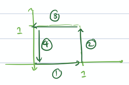
The four numbered parameterizations travel counterclockwise around the unit square.
A common parameterization is to use arc length as $t$. We can use interpolation on parameterized curves $x(t)$ and $y(t)$ as well.
Given $(x_i,y_i)$ data points, parameterize $t_i$ with $(x_0,y_0)$ and $(x_n,y_n)$ by:
- Use node index as parameterization, e.g. $t_i=i$.
- Approximate arc-length parameterization: set $t_0=0$ at the first node, then
We can apply curve concepts to surfaces by subdividing them.
An ordinary differential equation is a function $f$ relating a variable and its derivative:
\[y'(t)=f(t,y(t)).\]Question: Model a mouse population $y(t)$ over time $t$.
Answer:
- With enough food, say the population changes as $y’(t)=ay(t)$, where $a$ is constant. Suppose $y_0=y(t_0)$. Then
Proof:
\[y'(t)=y_0e^{a(t-t_0)}a=ay_0e^{a(t-t_0)}=ay(t).\]This is exponential growth in population.
- With food constraints modelled by $b$,
Notice the population drops as $y(t)>a/b$. Suppose $y_0=y(t_0)$. The closed form is
\[y(t)=\frac{ay_0e^{a(t-t_0)}}{by_0e^{a(t-t_0)}+(a-y_0b)},\]which is logistic population growth.
- Another model:
There is no general closed-form solution.
Most ODEs are too complex to have simple closed forms, so we develop methods to find approximates $(t_i,y_i)$ where $y_i\approx y(t_i)$. Given $(t_i,y_i)$ pairs, use interpolation methods to derive a full solution for all times.
Initial-value problem (IVP):
\[y'(t)=f(t,y(t))\quad\text{(dynamics function, in standard form)},\] \[y(t_0)=y_0\quad\text{(initial condition)}.\]Find/approximate $y(t)$.
Time-stepping: Given initial conditions, step to the next time endpoint using the dynamics function and time step $h$.
Set $n=0$, $t=t_0$, $y=y_0$:
- Compute $y_{n+1}$.
- Increment time, $t_{n+1}=t_n+h$.
- Advance $n=n+1$.
Forward Euler
- Single-step: use information from the current time only.
- Multistep: use information from previous steps.
- Implicit: solve the given function to find $y_{n+1}$.
- Explicit: evaluate the given function for $y_{n+1}$.
- Time step $h$ can be constant or vary.
Explicit, single-step scheme; more accurate as $h\to0$.
\[y_n'=f(t_n,y_n),\] \[y_{n+1}=y_n+hy_n'=y_n+hf(t_n,y_n).\]Question: For $y’(t)=2y(t)$, $t_0=1$, $y(t_0)=3$:
- Write the FE recurrence for $h=1$ and $h=1/2$.
- Use FE to approximate $y$ at $t=4$.
- Compare against $y(t)=3e^{2(t-t_0)}$.
Answer:
\[h=1:\quad y_{n+1}=y_n+2y_n=3y_n.\] \[h=\frac12:\quad y_{n+1}=y_n+y_n=2y_n.\] \[\begin{array}{c|c|c||c|c|c} n&t&y_n(h=1)&n&t&y_n(h=1/2)\\\hline 0&1&3&0&1&3\\ 1&2&9&1&1.5&6\\ 2&3&27&2&2&12\\ 3&4&81&3&2.5&24\\ &&&4&3&48\\ &&&5&3.5&96\\ &&&6&4&192 \end{array}\]The true value is $y(4)\approx1210.3$. Notice $81$ and $192$ are both terrible approximations, but $192$ is better.
ODEs - Forward Euler
We can think of time stepping as finding an approximate integral for $y’$, since we approximate $y$ and
\[y=\int y'\,dt.\]Geometrically, FE approximates using the tangent height $f(t_n,y_n)$:
\[y_{n+1}=y_n+hf(t_n,y_n).\]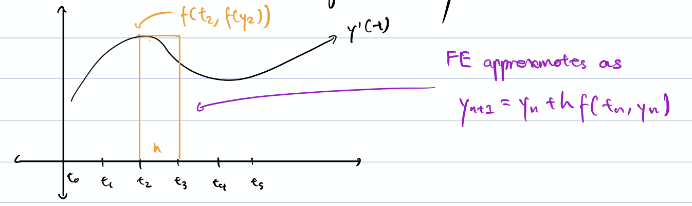
A smooth solution curve with a Forward Euler step of width $h$, using the slope $f(t_2,y(t_2))$ to approximate the next value.
FE applies to systems:
\[x'(t)=f_x(t,x(t),y(t)),\quad x(t_0)=x_0,\] \[y'(t)=f_y(t,x(t),y(t)),\quad y(t_0)=y_0.\]In vector notation,
\[\begin{bmatrix}x_{n+1}\\y_{n+1}\end{bmatrix} =\begin{bmatrix}x_n\\y_n\end{bmatrix} +h\begin{bmatrix}f_x(t_n,x_n,y_n)\\f_y(t_n,x_n,y_n)\end{bmatrix}.\]Example:
\[\begin{bmatrix}x_{n+1}\\y_{n+1}\end{bmatrix} =\begin{bmatrix}x_n\\y_n\end{bmatrix} +h\begin{bmatrix}-ay_n+\sin t_n\\x_n\end{bmatrix}, \qquad \begin{bmatrix}x_0\\y_0\end{bmatrix} =\begin{bmatrix}2\\3\end{bmatrix}.\]Question: For a particle with $x’=-y$, $y’=x$, $x(0)=2$, $y(0)=0$, write FE with $h=2$ and apply it to $t=6$.
Answer:
\[\begin{bmatrix}x_{n+1}\\y_{n+1}\end{bmatrix} =\begin{bmatrix}x_n\\y_n\end{bmatrix} +2\begin{bmatrix}-y_n\\x_n\end{bmatrix} =\begin{bmatrix}x_n-2y_n\\2x_n+y_n\end{bmatrix}.\] \[\begin{array}{c|c|c|c} n&t&x_n&y_n\\\hline 0&0&2&0\\ 1&2&2&4\\ 2&4&-6&8\\ 3&6&-22&-4 \end{array}\]This gives another very bad approximation.
Recall the Taylor series
\[f(x)=f(a)+f'(a)(x-a)+\frac{f''(a)}{2!}(x-a)^2+\frac{f'''(a)}{3!}(x-a)^3+\cdots.\]It approximates a function by knowing $f(a)$ and derivatives at $x=a$.
Deriving FE, 1: Approximate $y’$ using a finite difference:
\[y'(t_n)=\frac{y_{n+1}-y_n}{t_{n+1}-t_n}.\]Since $y’(t_n)=f(t_n,y(t_n))$,
\[f(t_n,y(t_n))=\frac{y_{n+1}-y_n}{t_{n+1}-t_n}=\frac{y_{n+1}-y_n}{h},\]so
\[y_{n+1}=hf(t_n,y(t_n))+y_n.\]Deriving FE, 2: Approximate $y’$ with a simplified Taylor series. Center at $t_n$ and evaluate at $t_{n+1}$:
\[y(t_{n+1})=y(t_n)+hy'(t_n)+\frac{h^2}{2!}y''(t_n)+\cdots.\]Dropping $h^2$ and above,
\[y_{n+1}\approx y_n+hy'(t_n)=y_n+hf(t_n,y_n).\]Absolute/global error at step $n$ is $\lvert y_n-y(t_n)\rvert$. We do not know $y(t_n)$, so approximate it using Taylor series.
Local truncation error is the error at each step.
Error of Forward Euler:
\[y_{n+1}=y_n+hf(t_n,y_n).\]The Taylor series centered at $t_n$ and evaluated at $t_{n+1}$ is
\[y(t_{n+1})=y(t_n)+hy'(t_n)+\frac{h^2}{2}y''(t_n)+O(h^3).\]Assuming exact data at $t_n$, local error is the difference between FE and the Taylor series.
\[\begin{aligned} y_{n+1}-y(t_{n+1}) &=y_n+hy'(t_n)-\left(y(t_n)+hy'(t_n)+\frac{h^2}{2}y''(t_n)+O(h^3)\right)\\ &=-\frac{h^2}{2}y''(t_n)-O(h^3)=O(h^2). \end{aligned}\]Thus local error of FE is $O(h^2)$.
Trapezoidal: keep the $y’‘(t_n)$ term, approximating
\[y''(t_n)=\frac{y'(t_{n+1})-y'(t_n)}h+O(h).\]Then
\[y_{n+1}=y_n+\frac h2[f(t_{n+1},y_{n+1})+f(t_n,y_n)],\]with $O(h^3)$ LTE. Intuition: evaluate slope at both ends and step according to average slope. Trapezoidal is implicit because it requires $f(t_{n+1},y_{n+1})$.
Explicit schemes are simpler/faster per step and less stable. Implicit schemes are more complex/expensive per step and more stable, so can use larger time steps.
Improved Euler: avoid implicitness by estimating the endpoint with FE:
\[y_{n+1}^*=y_n+hf(t_n,y_n),\] \[y_{n+1}=y_n+\frac h2[f(t_n,y_n)+f(t_{n+1},y_{n+1}^*)],\]with LTE $O(h^3)$.
ODEs - More Schemes
Recall multivariable Taylor expansion:
\[f(x+h_x,y+h_y)=f(x,y)+h_xf_x+h_yf_y+O(h_x^2)+O(h_y^2).\]Beginning with
\[y(t_{n+1})=y(t_n)+hy'(t_n)+\frac{h^2}{2}y''(t_n)+O(h^3),\]and using
\[y''(t_n)=\frac{y'(t_{n+1})-y'(t_n)}h+O(h),\]gives
\[y_{n+1}=y_n+\frac h2[y'(t_n)+y'(t_{n+1})]+O(h^3),\]which is the trapezoidal rule.
For Improved Euler, use the FE estimate $y_{n+1}^*=y_n+hf(t_n,y_n)$ and expand $f$ in the $y$ variable:
\[f(t_{n+1},y_{n+1})=f(t_{n+1},y_{n+1}^*)+O(h^2).\]Substitution in trapezoidal gives the explicit Improved Euler formula with $O(h^3)$ LTE.
Question: Apply Improved Euler to $x’=-y$, $y’=x$, $x(0)=2$, $y(0)=0$, with $h=2$ to find $(x,y)$ at $t=4$. Also write time-stepping equations for trapezoidal.
Answer:
For Improved Euler,
\[\begin{aligned} x_{n+1}^*&=x_n-2y_n,& y_{n+1}^*&=y_n+2x_n,\\ x_{n+1}&=x_n-(y_n+y_{n+1}^*),& y_{n+1}&=y_n+(x_n+x_{n+1}^*). \end{aligned}\] \[\begin{array}{c|c|c|c} n&t&x_n&y_n\\\hline 0&0&2&0\\ 1&2&-2&4\\ 2&4&-6&-8 \end{array}\]Generic trapezoidal:
\[y_{n+1}=y_n+\frac h2[f(t_n,y_n)+f(t_{n+1},y_{n+1})].\]For the system,
\[x_{n+1}=x_n-\frac h2(y_n+y_{n+1}),\] \[y_{n+1}=y_n+\frac h2(x_n+x_{n+1}).\]Backward Euler: Forward Euler, but take the height at $t_{n+1}$ instead of $t_n$, making it implicit; LTE $O(h^2)$:
\[y_{n+1}=y_n+hf(t_{n+1},y(t_{n+1})).\]Remember sign of $h$ alternates [when deriving backward differences].
Runge-Kutta
RK2 / midpoint: Take an FE step to the halfway point, evaluate slope there as $k_2$, then use it to take a full step:
\[k_1=hf(t_n,y_n),\] \[k_2=hf\left(t_n+\frac h2,y_n+\frac{k_1}{2}\right),\] \[y_{n+1}=y_n+k_2.\]Equivalently,
\[y_{n+1/2}=y_n+\frac h2f(t_n,y_n),\] \[y_{n+1}=y_n+hf(t_n+h/2,y_{n+1/2}).\]LTE is $O(h^3)$.
Fourth-order Runge-Kutta: Evaluate $y’(t)=f(t,y)$ at intermediate positions $k_1,\ldots,k_4$ and combine to find $y_{n+1}$. Fits a quadratic; LTE $O(h^5)$.
\[\begin{aligned} k_1&=hf(t_n,y_n),\\ k_2&=hf(t_n+h/2,y_n+k_1/2),\\ k_3&=hf(t_n+h/2,y_n+k_2/2),\\ k_4&=hf(t_n+h,y_n+k_3),\\ y_{n+1}&=y_n+\frac16(k_1+2k_2+2k_3+k_4). \end{aligned}\]For constant step $h$, number of steps is $O(h^{-1})$. Therefore global error is local error times all steps, so the global order is one degree less:
\[\begin{array}{lll} \text{FE:}&O(h^2)O(h^{-1})=O(h),&\text{first-order accurate},\\ \text{Trapezoidal:}&O(h^3)O(h^{-1})=O(h^2),&\text{second-order accurate},\\ \text{RK4:}&O(h^5)O(h^{-1})=O(h^4),&\text{fourth-order accurate}. \end{array}\]Backward Differentiation Formulas
BDF1, BDF2, etc.; the number indicates global-error order. Generalizes Backward Euler using previous time steps.
\[\text{BDF1:}\quad y_{n+1}=y_n+hf(t_{n+1},y_{n+1}),\] \[\text{BDF2:}\quad y_{n+1}=\frac43y_n-\frac13y_{n-1}+\frac23hf(t_{n+1},y_{n+1}).\]Derive by interpolation:
- Fit an interpolant $p(t)$ with Lagrange polynomials to unknown $(t_{n+1},y_{n+1})$ and one or more earlier points.
- Determine $p’(t)$ by differentiating.
- Require endpoint slope to match: $p’(t_{n+1})=f(t_{n+1},y_{n+1})$.
- Rearrange for BDF.
For BDF1, fit $(t_n,y_n)$ and $(t_{n+1},y_{n+1})$:
\[p(t)=y_n\frac{t-t_{n+1}}{t_n-t_{n+1}}+y_{n+1}\frac{t-t_n}{t_{n+1}-t_n}.\]Then
\[p'(t_{n+1})=\frac{y_{n+1}-y_n}{t_{n+1}-t_n}=f(t_{n+1},y_{n+1}),\]so $y_{n+1}=y_n+hf(t_{n+1},y_{n+1})$.
For BDF2, fit $(t_{n-1},y_{n-1})$, $(t_n,y_n)$, $(t_{n+1},y_{n+1})$. At $t_{n+1}$,
\[p'(t_{n+1})=\frac1{2h}y_{n-1}-\frac2h y_n+\frac3{2h}y_{n+1}.\]Set equal to $f(t_{n+1},y_{n+1})$ and rearrange to obtain BDF2.
Second-order Adams-Bashforth: explicit, multistep, LTE $O(h^3)$:
\[y_{n+1}=y_n+\frac32hf(t_n,y_n)-\frac12hf(t_{n-1},y_{n-1}).\]Scheme summary:
\[\begin{array}{l|l|l|l} \text{scheme}&\text{step}&\text{explicit/implicit}&\text{global error}\\\hline \text{Forward Euler}&\text{single}&\text{explicit}&O(h)\\ \text{Improved Euler}&\text{single}&\text{explicit}&O(h^2)\\ \text{Midpoint/RK2}&\text{single}&\text{explicit}&O(h^2)\\ \text{RK4}&\text{single}&\text{explicit}&O(h^4)\\ \text{Trapezoidal/Improved Euler}&\text{single}&\text{implicit/explicit}&O(h^2)\\ \text{Backward Euler/BDF1}&\text{single}&\text{implicit}&O(h)\\ \text{BDF2}&\text{multi}&\text{implicit}&O(h^2)\\ \text{2-step Adams-Bashforth}&\text{multi}&\text{explicit}&O(h^2)\\ \text{3rd-order Adams-Moulton}&\text{multi}&\text{implicit}&O(h^3) \end{array}\]ODEs - Higher-Order Systems and Stability
Order of an ODE: highest derivative appearing in it. Convert higher-order ODEs into first-order ODEs:
- For each variable $y$ with more than a first derivative, introduce $y_i=y^{(i-1)}$ for $i=1$ to $n$.
- Substitute new $y_i$’s into the original ODE.
- Relate the $y_i$’s through new equations.
Question: Convert $y’‘(t)=ty(t)$, $y(1)=1$, $y’(1)=2$ to a first-order system.
Answer:
\[y_2=y',\quad y_1=y,\] \[y_2'=ty_1,\quad y_1'=y_2,\]with $y_2(1)=2$, $y_1(1)=1$.
Question: Convert
\[y^{(5)}(t)-3y'(t)y'''(t)+\sin(t)y''(t)-t[y^{(4)}(t)]^2=e^t\]to a first-order ODE.
Answer: Let $y_5=y^{(4)}$, $y_4=y’’’$, $y_3=y’’$, $y_2=y’$, $y_1=y$. Then
\[y_5'=e^t+3y_2y_4-\sin(t)y_3+t(y_5)^2,\] \[y_4'=y_5,\quad y_3'=y_4,\quad y_2'=y_3,\quad y_1'=y_2.\]Question: Convert
\[x''+y'x+2t=0,\] \[y''+(y')^2x+t=0\]to four first-order equations.
Answer: Let $x_2=x’$, $x_1=x$, $y_2=y’$, $y_1=y$:
\[x_2'=-y_2x_1-2t,\quad x_1'=x_2,\] \[y_2'=-(y_2)^2x_1-t,\quad y_1'=y_2.\]Unstable: error $\epsilon$ in initial conditions leads to error growing exponentially as steps $n\to\infty$.
Use the test equation $y’=-\lambda y$. Exact $y(t)=y_0e^{-\lambda t}\to0$ as $t\to\infty$. A numerical approximation should also have $y_n\to0$.
To test stability: apply a time-stepping scheme, find a closed form for solution/error behaviour, and find conditions on $h$ ensuring error approaches zero.
ODEs - Stability and Truncation Error
For Forward Euler on $y’=-\lambda y$, $\lambda>0$:
\[y_{n+1}=y_n(1-h\lambda),\qquad y_n=(1-h\lambda)^ny_0.\]It goes to zero only when
\[|1-h\lambda|<1\Longleftrightarrow0<h\lambda<2.\]If $y(t_0)=y_0+E_0$, then
\[E_n=(1-h\lambda)^nE_0.\]FE is conditionally stable.
For Backward Euler,
\[y_{n+1}=y_n-h\lambda y_{n+1},\] \[y_{n+1}=\frac1{1+h\lambda}y_n,\qquad y_n=\frac1{(1+h\lambda)^n}y_0.\]For $\lambda>0,h>0$, both solution and error go to zero. BE is stable.
For Improved Euler,
\[y_{n+1}^*=y_n(1-h\lambda),\] \[y_{n+1}=y_n\left(1-h\lambda+\frac{h^2\lambda^2}{2}\right).\]Stability requires
\[\left|1-h\lambda+\frac{h^2\lambda^2}{2}\right|<1,\]which gives $0<h\lambda<2$, as in FE. It has the same stability range for this problem even though LTE is $O(h^3)$.
For linear test equations, the bound relates to $h\lvert f_y\rvert$, e.g. $\lvert h(-a)\rvert<1$ for $y’=-ay$. For nonlinear problems it depends on $f_y$ at some point. For systems it depends on eigenvalues of the Jacobian
\[J(y_1,\ldots,y_n)=\left[\frac{\partial f_i}{\partial y_j}\right].\]To find local truncation error for $y_{n+1}=\mathrm{RHS}$:
- Replace approximations on RHS with exact versions, e.g. $y_n\to y(t_n)$ and $f(t_{n+1},y_{n+1})\to y’(t_{n+1})$.
- Taylor-expand all RHS quantities about $t_n$.
- Taylor-expand exact $y(t_{n+1})$ to compare.
- Compute $y(t_{n+1})-y_{n+1}$. Lowest-degree non-cancelling power of $h$ gives LTE.
For FE,
\[y_{n+1}=y(t_n)+hy'(t_n),\]whereas
\[y(t_{n+1})=y(t_n)+hy'(t_n)+\frac{h^2}{2}y''(t_n)+\cdots,\]so LTE is $\frac{h^2}{2}y’‘(t_n)=O(h^2)$.
For trapezoidal,
\[y_{n+1}=y(t_n)+\frac h2[y'(t_n)+y'(t_{n+1})].\]Taylor-expanding $y’(t_{n+1})$ gives
\[y_{n+1}=y(t_n)+hy'(t_n)+\frac{h^2}{2}y''(t_n)+O(h^3),\]so LTE is $O(h^3)$.
For BDF2,
\[y_{n+1}=\frac43y(t_n)-\frac13y(t_{n-1})+\frac23hy'(t_{n+1}).\]Using
\[y(t_{n-1})=y(t_n)-hy'(t_n)+\frac{h^2}{2}y''(t_n)-\frac{h^3}{6}y'''(t_n)+O(h^4),\] \[y'(t_{n+1})=y'(t_n)+hy''(t_n)+\frac{h^2}{2}y'''(t_n)+O(h^3),\]gives
\[y_{n+1}=y(t_n)+hy'(t_n)+\frac{h^2}{2}y''(t_n)+\frac49h^3y'''(t_n)+O(h^4).\]Comparing with Taylor, the difference is $O(h^3)$.
Adaptive Time Stepping
Smaller time steps mean less error but larger computational cost. Vary $h$ with adaptive time stepping:
- Compute approximate solutions with two schemes of different orders.
- Estimate error by taking their difference.
- While error $>$ tolerance, set $h:=h/2$ and recompute.
- Estimate the error coefficient and predict a good next step $h_{\text{new}}$.
- Repeat until end time.
At the same time, let
\[y_{n+1}^{(A)}=y(t_{n+1})+Ch^p+O(h^{p+1}),\] \[y_{n+1}^{(B)}=y(t_{n+1})+O(h^{p+1}).\]Then
\[|y_{n+1}^{(A)}-y_{n+1}^{(B)}|=Ch^p+O(h^{p+1}),\]so the dominant term matches method A’s true error.
Estimate
\[C\approx\frac{|y_{n+1}^{(A)}-y_{n+1}^{(B)}|}{h_{\text{old}}^p}.\]Assume $C$ changes slowly. Set
\[\mathrm{err}_{\text{next}}\approx C(h_{\text{new}})^p=\mathrm{tol}\]and solve:
\[h_{\text{new}}=h_{\text{old}}\left(\frac{\mathrm{tol}}{|y_{n+1}^{(A)}-y_{n+1}^{(B)}|}\right)^{1/p}.\]Scale this back by a factor, e.g. $1/2$ or $3/4$, because the estimate will not be exact.
Stiff problem: an interesting aspect of the solution changes slowly, so we want big time steps, but a stability condition forces small time steps. Time-stepping schemes designed for this are called stiff solvers.
Fourier Transforms - Introduction
Fourier analysis:
- Apply a Fourier transform to discrete data or a continuous function in the time/space domain to get Fourier form in the frequency domain.
- Process/analyze in the frequency domain, e.g. sharpen an image.
- Transform back.
For a continuous Fourier series,
\[f(t)=a_0+\sum_{k=1}^{\infty}a_k\cos(kt)+\sum_{k=1}^{\infty}b_k\sin(kt).\]$a_k,b_k$ indicate amplitude for period $2\pi/k$ or frequency $k/(2\pi)$.
Orthogonality identities over $[0,2\pi]$:
\[\int_0^{2\pi}\cos(kt)\sin(jt)\,dt=0,\] \[\int_0^{2\pi}\cos(kt)\cos(jt)\,dt=0\quad(k\neq j),\] \[\int_0^{2\pi}\sin(kt)\sin(jt)\,dt=0\quad(k\neq j),\] \[\int_0^{2\pi}\sin(kt)\,dt=0,\qquad\int_0^{2\pi}\cos(kt)\,dt=0.\]To determine $a_0$, integrate over $2\pi$:
\[\int_0^{2\pi}f(t)\,dt=2\pi a_0,\]so $a_0=(2\pi)^{-1}\int_0^{2\pi}f(t)\,dt$, the average value. Multiplying by $\cos(\ell t)$ or $\sin(\ell t)$ and integrating isolates
\[a_\ell=\frac{\int_0^{2\pi}f(t)\cos(\ell t)\,dt}{\int_0^{2\pi}\cos^2(\ell t)\,dt}, \qquad b_\ell=\frac{\int_0^{2\pi}f(t)\sin(\ell t)\,dt}{\int_0^{2\pi}\sin^2(\ell t)\,dt}.\]For $z=a+bi$, $\bar z=a-bi$, $\lvert z\rvert=\sqrt{a^2+b^2}$, and $\arg z=\operatorname{atan2}(b,a)$. Euler’s formula is $e^{i\theta}=\cos\theta+i\sin\theta$, hence
\[\cos\theta=\frac{e^{i\theta}+e^{-i\theta}}2,\qquad \sin\theta=\frac{e^{i\theta}-e^{-i\theta}}{2i}.\]Complex Fourier form:
\[f(t)=\sum_{k=-\infty}^{\infty}c_ke^{ikt},\qquad c_k=\frac1{2\pi}\int_0^{2\pi}e^{-ikt}f(t)\,dt.\]For $k>0$, $c_k=(a_k-ib_k)/2$, $c_{-k}=(a_k+ib_k)/2$, and $c_0=a_0$. $\lvert c_k\rvert$ is amplitude and $\arg(c_k)$ is phase. Truncate to $-M\leq k\leq M$ for an approximation.
Discrete Fourier Transform
Suppose $f_n=f(t_n)$ for $N$ points, $t_n=2\pi n/N$, with $N$ even. The inverse discrete Fourier transform approximates
\[f_n=\sum_{k=0}^{N-1}F_k\omega^{nk},\qquad\omega=e^{2\pi i/N}.\]The $\omega^k$ are the $N$th roots of unity. Define coefficients periodically, $F_{j+N}=F_j$.
Orthogonality:
\[\sum_{j=0}^{N-1}\omega^{j(k-\ell)}=N\delta_{k\ell}.\]For $k=\ell$, the sum is $N$. Otherwise, use the geometric-series identity and $\omega^{N(k-\ell)}=1$ to get zero.
Multiply the inverse relation by $\omega^{-nk}$ and sum over $n$ to isolate the DFT:
\[F_k=\frac1N\sum_{n=0}^{N-1}f_n\omega^{-nk}.\]Question: Perform IDFT on $F=[-2,2+i,-2,2-i]$, $N=4$, $\omega=e^{2\pi i/4}=i$.
Answer:
\[f_0=0,\qquad f_1=-2,\qquad f_2=-8,\qquad f_3=2.\]Question: For $f_n=\cos(2\pi n/N)$, show $F_1=F_{N-1}=1/2$ and all other $F_k=0$.
Answer: Using $\cos\theta=(e^{i\theta}+e^{-i\theta})/2$ and orthogonality,
\[F_k=\frac1{2N}\sum_{n=0}^{N-1}\left(\omega^{n(1-k)}+\omega^{-n(1+k)}\right) =\frac12\delta_{k,1}+\frac12\delta_{k,N-1}.\]DFT properties:
- ${F_k}$ is doubly infinite and periodic with period $N$: if $k=mN+p$, then $\omega^{-k}=\omega^{-p}$ and $F_k=F_p$.
- Conjugate symmetry: for real data, $\overline{F_k}=F_{N-k}$, using $\overline{\omega^j}=\omega^{-j}$.
Power spectrum: plot $\lvert F_k\rvert$. A smooth bump indicates one dominant frequency; a rough bump indicates more active frequencies; symmetry indicates real data.
In matrix form $F=Mf$, where the $k$th row is $N^{-1}[1,\omega^{-k},\ldots,\omega^{-(N-1)k}]$. Orthogonality gives $M^TM=I/N$, so $M^{-1}=NM^T$ [with conjugation understood for the complex matrix]. Thus IDFT is $f=M^{-1}F$.
Fast Fourier Transform Derivation
Slow Fourier transform costs $O(N^2)$: for each $k$, sum all $N$ samples.
For the FFT, rewrite one DFT as two half-length DFTs:
\[F_k=\frac1N\sum_{n=0}^{N/2-1}(f_n+f_{n+N/2}\omega^{-Nk/2})\omega^{-nk}.\]Since $\omega^{-Nk/2}=(-1)^k$,
\[F_{2j}=\frac1N\sum_{n=0}^{N/2-1}(f_n+f_{n+N/2})(\omega^2)^{-nj},\] \[F_{2j+1}=\frac1N\sum_{n=0}^{N/2-1}(f_n-f_{n+N/2})\omega^{-n}(\omega^2)^{-nj}.\]Define $g_n=(f_n+f_{n+N/2})/2$ and $h_n=(f_n-f_{n+N/2})\omega^{-n}/2$. Then $F_{2j}=G_j$ and $F_{2j+1}=H_j$, two DFTs of length $N/2$. Each stage applies even/odd splitting; bit-reverse the output to recover original indices. This works when $N$ is a power of two.
Splitting costs $O(N)$ per stage, and $N=2^m$ gives $m=\log_2N$ stages, hence $O(N\log N)$. The inverse transform has the same form, with signs reversed and the corresponding normalization.
Question: Perform FFT on $[1,2,3,4,1,2,3,4]$.
Answer: The notes carry the vector through three butterfly stages ($N=8,4,2$), pairing the repeated halves; the final coefficients are assembled from the even and odd transforms.
Two-Dimensional FFT and Aliasing
For a one-dimensional grayscale image, take DFT of pixel values. For compression, throw away $F_k$ where $\lvert F_k\rvert<\text{tol}$, then reconstruct with IDFT.
For an $N\times M$ image,
\[F_{k,\ell}=\frac1{NM}\sum_{n=0}^{N-1}\sum_{j=0}^{M-1}f_{n,j}\omega_N^{-nk}\omega_M^{-j\ell}.\]Apply FFT to each of $M$ rows, costing $O(MN\log N)$, then each of $N$ columns, costing $O(NM\log M)$: total $O(MN\log(MN))$. Divide images into blocks for compression because pixels in a block often have similar data.
Aliasing: a high-frequency signal appears as low frequency due to sample spacing. Anti-aliasing filters high frequencies. Sampling rate is $f_s=N/T$ samples/second; Fourier frequency is $k/T$ cycles/second.
Sampling the continuous series at $t_n=nT/N$ gives $f_n=\sum_kc_k\omega^{nk}$. Substituting into the DFT and using orthogonality gives
\[F_k=c_k+c_{k+N}+c_{k-N}+c_{k+2N}+\cdots.\]Thus DFT coefficients sum Fourier-series coefficients including arbitrarily high frequencies.
Fourier Correlation Function
High frequencies outside $[-N/2,N/2]$ alias as low frequencies inside it. Once sampled, there is no way to distinguish aliased frequencies. Partial solutions:
- Increase sampling rate.
- Filter before sampling to remove high frequencies, e.g. optical low-pass filter.
For two real periodic data sets $y_i,z_i$, define circular correlation
\[\phi_n=\frac1N\sum_{i=0}^{N-1}y_{i+n}z_i.\]The maximizing $n$ shifts $y$ into maximum dot product with $z$.
Question: For $[1,2,3,4,0,3,4]$ and $[0,2,4,2,1,2,4]$, find $\phi_n$.
Answer: At $n=0$,
\[\phi_0=(1\cdot0+2\cdot2+3\cdot4+4\cdot2+0\cdot1+3\cdot2+4\cdot4)/7=46/7.\]Naively trying all shifts costs $O(N^2)$. With FFT:
- $Y=\operatorname{FFT}(y)$, $Z=\operatorname{FFT}(z)$: $O(N\log N)$.
- $\Phi_k=\overline{Y_k}Z_k$ for $k=0,\ldots,N-1$: $O(N)$.
- $\phi=\operatorname{IFFT}(\Phi)$: $O(N\log N)$.
The notes derive step 2 by substituting the inverse DFTs for $y_{i+n}$ and $z_i$ into the correlation DFT and applying roots-of-unity orthogonality.
Numerical PageRank
Degree: number of links leaving a node. Adjacency matrix: $G_{i,j}=1$ if link $i\to j$ exists and $0$ otherwise. Degree of node $i$ is the sum of entries in its column [under the transition-matrix orientation used here].
Heuristics: nodes with lots of incoming links, and nodes related to nodes with lots of incoming links, are important.
Random-surfer model: Start at some page and follow links at random for $K$ steps. Rank page $i$ by visits$(i)$/total visits. Problems: cycles, dead ends, and large $K$.
Define
\[P_{j,i}=\begin{cases}1/\deg(i),&i\to j,\\0,&\text{otherwise}. \end{cases}\]Let $d_i=1$ if $\deg(i)=0$, otherwise $0$. Let $R$ be the number of pages and $e=(1,\ldots,1)^T$. Define
\[P'=P+\frac1R ed^T,\]so a dead end transitions to all pages with equal chance. Define
\[M=\alpha P'+(1-\alpha)\frac1R ee^T.\]The first term follows links without dead ends; the second teleports randomly to avoid cycles. $0\leq M_{i,j}\leq1$ and $\sum_iM_{i,j}=1$: properties of a Markov matrix.
Question: Construct $M$ for the displayed six-node directed web with $\alpha=1/2$.
Answer: First write $P$, $e$, and $d$, then add the uniform teleportation matrix.
For probability vector $p=(q_1,\ldots,q_R)^T$, $q_i\geq0$, $\sum_iq_i=1$,
\[p^{n+1}=Mp^n\]is the probability of being on each page after $n+1$ transitions. It remains a probability vector because entries are nonnegative and
\[\sum_i p_i^{n+1}=\sum_jp_j^n\sum_iM_{i,j}=1.\]We estimate $p^\infty=\lim_{k\to\infty}M^kp^0$; higher probability means greater importance.
p0 = e/R
for k = 1, ...
    pk = M p(k-1)
    if max_i |pk_i - p(k-1)_i| < tol, quit
Compute PageRank once and store it; keyword searches find matching pages and rank by $p^\infty$. Exploit sparsity without building dense $M$:
\[Mp^n=\alpha Pp^n+\frac\alpha R e(d^Tp^n)+\frac{1-\alpha}{R}e(e^Tp^n).\]Since $e^Tp^n=1$, the final term is $(1-\alpha)e/R$.
Eigenvalues/Eigenvectors Review
To incorporate other factors, use
\[M=\alpha(P+vd^T)+(1-\alpha)ve^T,\]where $v$ places extra weight on preferred sites.
An eigenvalue/eigenvector satisfies $Qx=\lambda x$, or $(\lambda I-Q)x=0$. A nonzero solution requires $\det(\lambda I-Q)=0$.
Question: For $Q=\begin{bmatrix}2&2\5&-1\end{bmatrix}$, find its eigenvalues and eigenvectors.
Answer:
\[\det(\lambda I-Q)=\lambda^2-\lambda-12=(\lambda-4)(\lambda+3).\]For $\lambda=4$, eigenvectors are $c[1,1]^T$. For $\lambda=-3$, they are $c[-2/5,1]^T$, $c\neq0$.
Properties of Markov matrices:
- Every Markov matrix $Q$ has $1$ as an eigenvalue.
- Every eigenvalue satisfies $\lvert\lambda\rvert\leq1$, so $1$ is largest.
- $Q$ is positive if $Q_{i,j}>0$ for all $i,j$.
- If $Q$ is positive Markov, there is only one linearly independent eigenvector for $\lambda=1$.
For (1), $Q^Te=e$ because rows of $Q^T$ sum to one. Since $\det Q=\det Q^T$, $1$ is also an eigenvalue of $Q$. For (2), choose the largest-magnitude component $x_k$ of an eigenvector of $Q^T$:
\[|\lambda||x_k|=\left|\sum_jQ_{j,k}x_j\right| \leq\sum_jQ_{j,k}|x_j| \leq|x_k|\sum_jQ_{j,k}=|x_k|,\]so $\lvert\lambda\rvert\leq1$.
PageRank Convergence
If $M$ is positive Markov, PageRank converges uniquely for any $p^0$. Write $p^0=\sum_ic_ix_i$, with $\lvert\lambda_1\rvert\geq\lvert\lambda_2\rvert\geq\cdots$:
\[M^kp^0=\sum_ic_i\lambda_i^kx_i=c_1x_1+\sum_{i\geq2}c_i\lambda_i^kx_i.\]$\lambda_1=1$, and the other terms vanish. Uniqueness follows because two scalar multiples of the unique eigenvector cannot both be distinct probability vectors summing to one. Convergence rate is proportional to $\lvert\lambda_2\rvert$. In PageRank, $\alpha$ approximates $\lvert\lambda_2\rvert$; e.g. $0.85^{144}\approx10^{-8}$. Smaller $\alpha$ converges faster at the cost of accuracy due to more random jumps.
Numerical Linear Algebra
Solve $Ax=b$ by:
- Factor $PA=LU$, where $U$ is triangular: $O(n^3)$.
- Solve $Lz=Pb$ by forward substitution: $O(n^2)$.
- Solve $Ux=z$ by back substitution: $O(n^2)$.
LU factorization core:
for k = 1, ..., n
    for i = k+1, ..., n
        m_ik = a_ik / a_kk
        for j = k+1, ..., n
            a_ij = a_ij - m_ik a_kj
Store the multipliers inside $U$. The right-hand side is unnecessary for factoring; new $b$ values require only $O(n^2)$ triangular solves.
Forward substitution:
for i = 1, ..., n
    z_i = b_i
    for j = 1, ..., i-1
        z_i = z_i - L_ij z_j
Back substitution similarly proceeds from $i=n$ down to $1$ and divides by $U_{ii}$.
Division by zero or near zero causes large factors that magnify floating-point error. A permutation matrix is an identity matrix with rows swapped; partial pivoting swaps rows so the largest-magnitude entry in the current column is in the pivot row. The notes work a $PA=LU$ example and define FLOP as a floating-point addition, subtraction, multiplication, or division. Useful sums include $\sum_{i=1}^ni=n(n+1)/2$ and $\sum_{i=1}^ni^2=n(n+1)(2n+1)/6$.
Ignoring pivots,
\[M^{(n-1)}\cdots M^{(2)}M^{(1)}A=U,\]so
\[A=(M^{(1)})^{-1}\cdots(M^{(n-1)})^{-1}U=LU.\]The inverse of an elimination matrix negates its off-diagonal multiplier. Solving by explicitly computing $A^{-1}$ costs more and incurs more floating-point error: factor $A=LU$, solve $LUx=e_i$ for every identity column, then compute $x=A^{-1}b$.
Norms and Conditioning
Norm means size/magnitude:
\[\|x\|_1=\sum_i|x_i|\quad\text{(Manhattan)},\] \[\|x\|_2=\sqrt{\sum_ix_i^2}\quad\text{(Euclidean)},\] \[\|x\|_\infty=\max_i|x_i|,\]and generally $\lVert x\rVert_p=(\sum_i\lvert x_i\rvert^p)^{1/p}$.
Properties: $\lVert x\rVert=0\Leftrightarrow x=0$; $\lVert\alpha x\rVert=\lvert\alpha\rvert\lVert x\rVert$; $\lVert x+y\rVert\leq\lVert x\rVert+\lVert y\rVert$.
Matrix norm:
\[\|A\|=\max_{\|x\|=1}\|Ax\|.\] \[\|A\|_1=\max_j\sum_i|A_{i,j}|\quad\text{(maximum absolute column sum)},\] \[\|A\|_\infty=\max_i\sum_j|A_{i,j}|\quad\text{(maximum absolute row sum)},\] \[\|A\|_2=\sqrt{\lambda_{\max}(A^TA)},\] \[\|A\|_F=\sqrt{\sum_i\sum_jA_{i,j}^2}.\]Matrix-norm properties: positivity, homogeneity, triangle inequality, $\lVert Ax\rVert\leq\lVert A\rVert\lVert x\rVert$, $\lVert AB\rVert\leq\lVert A\rVert\lVert B\rVert$, and $\lVert I\rVert=1$.
For $Ax=b$, ask how perturbing $b$ or $A$ changes $x$.
Conditioning - Perturbing b
\[A(x+\delta x)=b+\delta b.\]Subtract $Ax=b$: $A\delta x=\delta b$, so $\delta x=A^{-1}\delta b$. From
\[\|b\|=\|Ax\|\leq\|A\|\|x\|\]and
\[\|\delta x\|\leq\|A^{-1}\|\|\delta b\|,\]obtain
\[\frac{\|\delta x\|}{\|x\|} \leq(\|A^{-1}\|\|A\|)\frac{\|\delta b\|}{\|b\|} =\kappa(A)\frac{\|\delta b\|}{\|b\|}.\]Conditioning - Perturbing A
\[(A+\delta A)(x+\delta x)=b.\]Expanding and subtracting $Ax=b$ gives
\[A\delta x=-\delta A(x+\delta x),\]so
\[\frac{\|\delta x\|}{\|x+\delta x\|} \leq\kappa(A)\frac{\|\delta A\|}{\|A\|}.\]Condition number $\kappa$ bounds relative change in $x$ due to relative change in $A$ or $b$. If $\kappa\approx1$, $A$ is well-conditioned; if $\kappa\gg1$, it is ill-conditioned. If unspecified, use the 2-norm. Norm equivalence: $C_1\lVert x\rVert_a\leq\lVert x\rVert_b\leq C_2\lVert x\rVert_a$.
Residual
\[r=b-Ax_{\text{approx}}.\]It stands in for error in $x$ and can be reduced until $r<$ tolerance. If $x_{\text{approx}}=x+\delta x$, then $A(x+\delta x)=b-r$, so
\[\frac{\|\delta x\|}{\|x\|}\leq\kappa(A)\frac{\|r\|}{\|b\|}.\]Question: Given $A$ and $A^{-1}$ in the notes, find $\kappa_1(A)$ and $\kappa_\infty(A)$.
Answer: Maximum column/row sums give $\kappa_1(A)=1\cdot3=3$ and $\kappa_\infty(A)=1\cdot3=3$.
If $Ax=\lambda x$, then $A^{-1}x=\lambda^{-1}x$: eigenvalues of $A^{-1}$ are reciprocals of those of $A$.
Question: What is $\kappa_2(A)$ if eigenvalues of $A^TA$ are $1,9,9$? Assume $A$ symmetric.
Answer:
\[\|A\|_2=\sqrt{\max_i\lambda_i(A^TA)}=\sqrt9=3.\]For $\lVert A^{-1}\rVert_2$, eigenvalues of
\[[A^{-1}]^TA^{-1}=(AA^T)^{-1}\]are $1,1/9,1/9$, since $A$ symmetric and $AA^T=A^TA$. Thus
\[\|A^{-1}\|_2=\sqrt1=1,\]and
\[\kappa_2(A)=3\cdot1=3.\]Exercises:
- Prove $\kappa(A^{-1})=\kappa(A)$:
- Prove $\kappa(A)\geq1$:
- Decide whether the displayed diagonal/near-diagonal example matrices are ill-conditioned or well-conditioned.